2021年10月 – ページ 4 – mowareのブログ 2nd

[Python] AI 06 手書き数字の認識不正解画像の表示

前回の続きです。

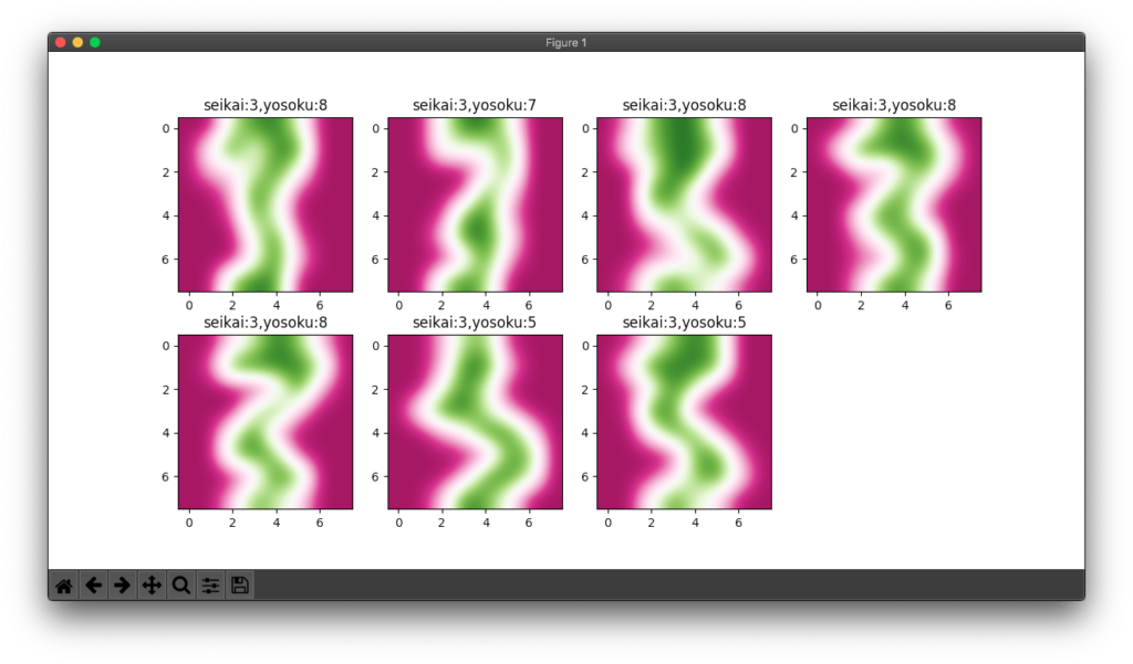
不正解が多かった3の該当画像を一括表示しました。確かに間違えやすい書き方だということが分かります。

from sklearn import datasets
import sklearn.svm as svm
import matplotlib.pyplot as plt

# 手書き数字のデータをロード
digits = datasets.load_digits()

# 画像データを変数all_featuresに、画像内容(数字)を変数teacher_labelsに格納
all_features = digits.data
teacher_labels = digits.target

num_samples = len(all_features)

model = svm.SVC(gamma = 0.001)

# 学習用の学習データと正解データ(1500個)
train_features=all_features[ : 1500 ]
train_teacher_labels=teacher_labels[ : 1500 ]
print(len(train_features))

# 検証用の学習データと正解データ(297個)
test_feature=all_features[1500 : ]
test_teacher_labels=digits.target[1500 : ]
print(len(test_feature))

# 学習実行
model.fit(train_features,train_teacher_labels)

# 数値予測データと検証用画像データ
predicted = model.predict(test_feature)
test_images = digits.images[1500 : ]

# 図のサイズ設定
fig = plt.figure(figsize=(12, 6))

# 前回記事で不正解が多かった3の画像で不正解のものを表示する
i = 1
for la,pre,img in zip(test_teacher_labels,predicted,test_images):
    if la == 3 and la != pre:
        plt.subplot(2, 4, i)
        plt.imshow(img, cmap='PiYG', interpolation='bicubic')
        plt.title(f'seikai:{la},yosoku:{pre}')
        i = i + 1

plt.show()

[Python] AI 05 手書き数字の認識 SVCによる予測

手書き数字の画像データ群を使ってSVCで学習させ、学習能力を検証しました。

digitsデータ1797個の内、1500個を学習、297個は検証に使いました。正解率は3の読み間違いが多いという結果でした。

ただdigits.dataというフラットなデータがあるにもかかわらず、何故わざわざ入れ子リストのdigits.imagesを平滑化するのかが分かりませんでした。

from sklearn import datasets
import sklearn.svm as svm
from sklearn.metrics import confusion_matrix
from sklearn.metrics import classification_report

# 手書き数字のデータをロード
digits = datasets.load_digits()

# 画像データを変数all_featuresに、画像内容(数字)を変数teacher_labelsに格納
all_features = digits.data
teacher_labels = digits.target

num_samples = len(all_features)

model = svm.SVC(gamma = 0.001)

# 学習用の学習データと教師データ(1500個)
train_features=all_features[ : 1500 ]
train_teacher_labels=teacher_labels[ : 1500 ]
print(len(train_features))

# 検証用の学習データと教師データ(297個)
test_feature=all_features[1500 : ]
test_teacher_labels=digits.target[1500 : ]
print(len(test_feature))

# 学習実行
model.fit(train_features,train_teacher_labels)

# 正解と数値予測データ
expected = test_teacher_labels
predicted = model.predict(test_feature)

print(f"分類機による分類結果 {model}: \n {classification_report(expected, predicted)} \n")

print(f"コンフュージョンマトリックス:\n {confusion_matrix(expected, predicted)}")
--------------------------------------------------

出力
--------------------------------------------------
1500
297
分類機による分類結果 SVC(gamma=0.001): 
               precision    recall  f1-score   support

           0       1.00      0.96      0.98        27
           1       0.97      1.00      0.98        31
           2       1.00      1.00      1.00        27
           3       0.96      0.77      0.85        30
           4       0.97      0.91      0.94        33
           5       0.91      1.00      0.95        30
           6       1.00      1.00      1.00        30
           7       0.97      1.00      0.98        30
           8       0.79      0.96      0.87        28
           9       1.00      0.94      0.97        31

    accuracy                           0.95       297
   macro avg       0.96      0.95      0.95       297
weighted avg       0.96      0.95      0.95       297
 

コンフュージョンマトリックス:
 [[26  0  0  0  1  0  0  0  0  0]
 [ 0 31  0  0  0  0  0  0  0  0]
 [ 0  0 27  0  0  0  0  0  0  0]
 [ 0  0  0 23  0  2  0  1  4  0]
 [ 0  0  0  0 30  0  0  0  3  0]
 [ 0  0  0  0  0 30  0  0  0  0]
 [ 0  0  0  0  0  0 30  0  0  0]
 [ 0  0  0  0  0  0  0 30  0  0]
 [ 0  1  0  0  0  0  0  0 27  0]
 [ 0  0  0  1  0  1  0  0  0 29]]

[Python] AI 04 手書き数字の認識データセット3D描画

手書き数字画像のデータセットについて64因子を3因子に減らし、3D散布図を描画しました。

分かりやすくするためとは言え、elifが8つも連なるようなコードは書かない方がいいと思います(教本P232)。AI専業であっても最低限のコーディング力は必要でしょう。

from sklearn import decomposition
from sklearn import datasets
import matplotlib.pyplot as plt

def getcolor(num):
    color_list = ['red','orange','yellow','greenyellow','green','cyan','blue','navy','purple','black']
    return color_list[num]

# 手書き数字のデータをロード
digits = datasets.load_digits()

# 画像データを変数all_featuresに、画像内容(数字)を変数teacher_labelsに格納
all_features = digits.data
teacher_labels = digits.target

# 主成分分析(3因子に減らす)
pca = decomposition.PCA(n_components=3)

# 64因子のall_featuresを3因子のthree_featuresに変換
three_features = pca.fit_transform(all_features)

# figureオブジェクト作成サイズを800＊800とする
fig = plt.figure(figsize=(8, 8))

# 1*1グリッドのサブプロット1に3D描画する
subfig = fig.add_subplot(111, projection = '3d')

# teacher_labelsに対応する色のリストを作成
colors = list(map(getcolor, teacher_labels))

# データの3Dカラー散布図描画設定
subfig.scatter(three_features[ : , 0 ], three_features[ : , 1 ], three_features[ : , 2 ], s=50, c=colors, alpha=0.3)

# グラフを表示
plt.show()

[Python] AI 03 手書き数字の認識

sklearnのdatesetsにあるdigitsという手書き数字の画像データを使ってデータの一部を表示しました。

今回はdigitsの最初の16個の画像データを4行*4列に並べました。

ここまで教本を読んで、スクリプトを書いた方のPython記述スキルが相当怪しいということが判明しました。あくまで対話式のPythonをある程度使えるAIの専門家なのでしょう。

なのでプログラミングの心得がある方は、スクリプトの意図を理解して自分でコードを書くのが賢明かと思います。

今回のスクリプトにしても意味不明な箇所があり、自分で整理すると13行が10行になりました(画像間の隙間調整は省略)。

from sklearn import datasets
import matplotlib.pyplot as plt

digits = datasets.load_digits()
ROWS_COUNT = 4
COLUMNS_COUNT = 4
DIGIT_GRAPH_COUNT = ROWS_COUNT * COLUMNS_COUNT

# figureオブジェクト作成サイズを1200*900に設定
fig = plt.figure(figsize=(12, 9)) 

for i in range(1, DIGIT_GRAPH_COUNT + 1):
    (fig.add_subplot(ROWS_COUNT, COLUMNS_COUNT, i)).imshow(digits.images[i],interpolation='bicubic', cmap='Set2')

plt.show()

[Python] AI 02 アヤメの分類超平面作成

前回の続きです。

アヤメの花弁データ(3列目と4列目)をサポートベクターマシン(SVM)を使って超平面で分類できるようにしました。

手順としては、データを標準化してからSVMのインスタンスを生成してモデル学習させ散布図を作成します。最後に適当な花弁データを入力してアヤメのどの種に該当するのか判定させています。

私の教本ではその前にデータを交差検証するために学習データと検証データに分けて、検証後に標準化データを結合して超平面を作成しています。

本の構成のためでしょうが、教本の方法は少々荒っぽいかと思います。統計学をかじったことのある方でしたら理由は分かるでしょう。

import numpy as np
import matplotlib.pyplot as plt
from mlxtend.plotting import plot_decision_regions as pdr
from sklearn import datasets
from sklearn.preprocessing import StandardScaler
from sklearn.svm import SVC

def test():
    model = analize()
    test_data=np.array([[3.0,4.0]])
    print(test_data)
    test_result = model.predict(test_data)
    print(test_result)
    plt.show()

def analize():
    iris = datasets.load_iris()

    features = iris.data[:,[2,3]]
    print(features)
    labels = iris.target

    sc = StandardScaler()
    sc.fit(features)

    # データの標準化(中心を0にするための変換)
    features_std = sc.transform(features)
    print(features_std)

    # 線形SVMのインスタンスを生成
    model = SVC(kernel='linear', random_state=None)

    # モデル学習
    model.fit(features_std, labels)

    fig = plt.figure(figsize=(12,8))

    # 散布図関連設定
    scatter_kwargs = {'s': 300, 'edgecolor': 'white', 'alpha': 0.5}
    contourf_kwargs = {'alpha': 0.2}
    scatter_highlight_kwargs = {'s': 200, 'label': 'Test', 'alpha': 0.7}
    
    pdr(features_std, labels, clf=model, scatter_kwargs=scatter_kwargs,
                        contourf_kwargs=contourf_kwargs,
                        scatter_highlight_kwargs=scatter_highlight_kwargs)

    return model

if __name__ == "__main__":
    test()
--------------------------------------------------

出力(検証データと判定結果のみ)
--------------------------------------------------
[[3. 4.]]
[2]

2021年10月
日	月	火	水	木	金	土
					1	2
3	4	5	6	7	8	9
10	11	12	13	14	15	16
17	18	19	20	21	22	23
24	25	26	27	28	29	30
31