[Python] AI 26 Keras学習モデル matplotlib詳細設定

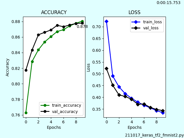
matplotlibの設定箇所が間延びした見た目だったのでスッキリさせました。

グラフ内と枠内にテキスト表示させています。val_accuracyの最後の値をグラフ内表示しています。枠内表示は実行時間とファイル名です。

start = time.time()

def plot_loss_accuracy_graph(history):
	process_time = time.time() - start
	td = datetime.timedelta(seconds = process_time)

	image ='accuracy_loss.png'

	fig = plt.figure(facecolor='#e0ffff')
	fig.subplots_adjust(bottom=0.15,wspace=0.3)

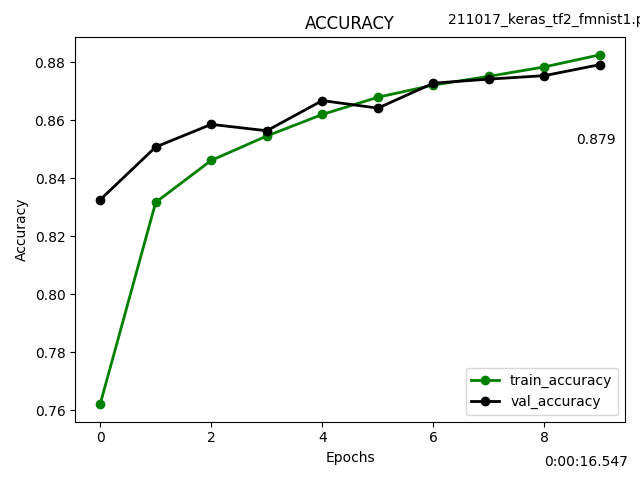
	ax = fig.add_subplot(121, title = 'ACCURACY',xlabel = 'Epochs',ylabel = 'Accuracy')
	ax.plot(history.history['accuracy'],"-o", color="green", label="train_accuracy", linewidth=2)
	ax.plot(history.history['val_accuracy'],"-o",color="black", label="val_accuracy", linewidth=2)
	ax.legend(loc="lower right")
	
	# グラフ内テキスト表示
	ax.text(len(history.history['val_accuracy']) -1, history.history['val_accuracy'][-1]-0.002, '{:.3f}'.format(history.history['val_accuracy'][-1]),verticalalignment='top',horizontalalignment='center')

	ax2 = fig.add_subplot(122, title = 'LOSS',xlabel = 'Epochs',ylabel = 'Loss')
	ax2.plot(history.history['loss'], "-D", color="blue", label="train_loss", linewidth=2)
	ax2.plot(history.history['val_loss'], "-D", color="black", label="val_loss", linewidth=2)
	ax2.legend(loc='upper right')

	# 枠内テキスト表示
	fig.text(0.68, 0.01, os.path.basename(__file__))
	fig.text(0.85, 0.97, str(td)[:11])

	fig.savefig(image)

[Python] AI 25 Keras学習モデル Fashion-MNIST

今回から教本はオライリー本 “scikit-learn, Keras, TensorFlowによる実践機械学習 第2版”になりました。10.2 KerasによるMLPの実装 から読み進めています。

ファッションアイテム画像のデータセットであるFashion-MNISTを使って識別学習させました。

訓練セットの画像データをX_trainと大文字で表記していますが、数学のルールで2次元配列は大文字、1次元配列は小文字になるからだそうです。

新しい教本ではデータセットを訓練セット、テストセット、検証セットの3種類に分けていました。私が目にしたネット情報では検証セットがないケースがほとんどでした。どちらがより適切なのかは不明ですが、今回は教本に従います。

import tensorflow.keras as keras
from tensorflow.keras import models
from keras.layers import Dense, Flatten
import matplotlib.pyplot as plt
import time,datetime,os,json

def plot_loss_accuracy_graph(history,val_accuracy):
	<略>
	return dt_now_str # 戻り値はグラフ作成日時

def main():
	epochs=10

	fashion_mnist = keras.datasets.fashion_mnist
	(X_train_full, y_train_full), (X_test, y_test) = fashion_mnist.load_data()

	print(f'X_train_full.shape {X_train_full.shape}')

	print(f'X_train_full.dtype {X_train_full.dtype}')

	X_valid, X_train = X_train_full[:5000] / 255., X_train_full[5000:] / 255.
	y_valid, y_train = y_train_full[:5000], y_train_full[5000:]
	X_test = X_test / 255.

	model = models.Sequential()
	model.add(Flatten(input_shape=[28, 28])) # 入力層
	model.add(Dense(300, activation="relu")) # Dense隠れ層
	model.add(Dense(100, activation="relu")) # Dense隠れ層
	model.add(Dense(10, activation="softmax")) # Dense出力層

	print(f'model.layers {model.layers}')

	model.summary()

	model.compile(loss="sparse_categorical_crossentropy",
				optimizer="sgd",
				metrics=["accuracy"])

	history = model.fit(X_train, y_train, epochs=epochs,
						validation_data=(X_valid, y_valid))
	print(f'history.history {history.history}')

	# 検証結果
	val_loss = history.history['val_loss'][-1]
	val_accuracy = history.history['val_accuracy'][-1]
	print('val_loss:', val_loss)
	print('val_accuracy:', val_accuracy)

	# 学習データ・グラフ化
	ret = plot_loss_accuracy_graph(history,val_accuracy)

	json_file = f'{ret}_history_data.json'
	with open(json_file ,'w' ) as f:
		json.dump(history.history ,f ,ensure_ascii=False ,indent=4)

	model.save(f'{ret}_keras-mnist-model.h5')

if __name__ == "__main__":
	main()