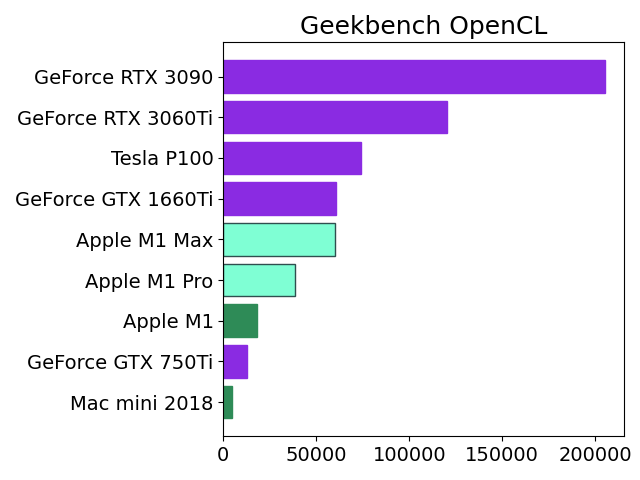
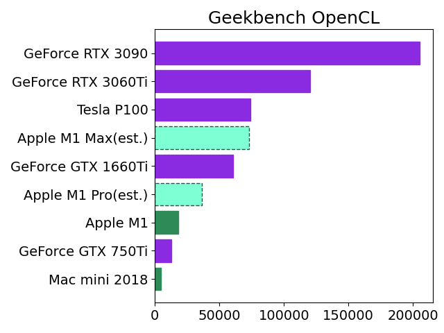
[Python] AI 25 Keras学習モデル Fashion-MNIST

今回から教本はオライリー本 “scikit-learn, Keras, TensorFlowによる実践機械学習 第2版”になりました。10.2 KerasによるMLPの実装 から読み進めています。

ファッションアイテム画像のデータセットであるFashion-MNISTを使って識別学習させました。

訓練セットの画像データをX_trainと大文字で表記していますが、数学のルールで2次元配列は大文字、1次元配列は小文字になるからだそうです。

新しい教本ではデータセットを訓練セット、テストセット、検証セットの3種類に分けていました。私が目にしたネット情報では検証セットがないケースがほとんどでした。どちらがより適切なのかは不明ですが、今回は教本に従います。

import tensorflow.keras as keras
from tensorflow.keras import models
from keras.layers import Dense, Flatten
import matplotlib.pyplot as plt
import time,datetime,os,json

def plot_loss_accuracy_graph(history,val_accuracy):
	<略>
	return dt_now_str # 戻り値はグラフ作成日時

def main():
	epochs=10

	fashion_mnist = keras.datasets.fashion_mnist
	(X_train_full, y_train_full), (X_test, y_test) = fashion_mnist.load_data()

	print(f'X_train_full.shape {X_train_full.shape}')

	print(f'X_train_full.dtype {X_train_full.dtype}')

	X_valid, X_train = X_train_full[:5000] / 255., X_train_full[5000:] / 255.
	y_valid, y_train = y_train_full[:5000], y_train_full[5000:]
	X_test = X_test / 255.

	model = models.Sequential()
	model.add(Flatten(input_shape=[28, 28])) # 入力層
	model.add(Dense(300, activation="relu")) # Dense隠れ層
	model.add(Dense(100, activation="relu")) # Dense隠れ層
	model.add(Dense(10, activation="softmax")) # Dense出力層

	print(f'model.layers {model.layers}')

	model.summary()

	model.compile(loss="sparse_categorical_crossentropy",
				optimizer="sgd",
				metrics=["accuracy"])

	history = model.fit(X_train, y_train, epochs=epochs,
						validation_data=(X_valid, y_valid))
	print(f'history.history {history.history}')

	# 検証結果
	val_loss = history.history['val_loss'][-1]
	val_accuracy = history.history['val_accuracy'][-1]
	print('val_loss:', val_loss)
	print('val_accuracy:', val_accuracy)

	# 学習データ・グラフ化
	ret = plot_loss_accuracy_graph(history,val_accuracy)

	json_file = f'{ret}_history_data.json'
	with open(json_file ,'w' ) as f:
		json.dump(history.history ,f ,ensure_ascii=False ,indent=4)

	model.save(f'{ret}_keras-mnist-model.h5')

if __name__ == "__main__":
	main()

[Python] AI 24 Keras学習モデル Custom train loop

Kerasのfit(), evaluate()を使わずforループで訓練する Custom train loopという方法で学習させてみました。

TensorFlowでは計算の高速化のためデータ型はfloat32を採用しています。そのためfloat64しか受け付けないjson.dumpを使う前には、float32からfloat64に変換しておく必要があります。

プログラマの習性でコードとしての整合性ばかり見がちなので、深層学習の理論も並行して身に付けるよう心掛けたいです。

import tensorflow as tf
from tensorflow.keras import models
from keras.layers import Dense, Dropout, Flatten
from keras.layers import Conv2D, MaxPooling2D
import matplotlib.pyplot as plt
import time,datetime,os
from stegano import lsb
import numpy as np
import json

def plot_loss_accuracy_graph(data):
	<略>
	return dt_now_str # 戻り値はグラフ作成日時

def create_model():
	model = models.Sequential()

	model.add(Conv2D(32, kernel_size=(3, 3),activation='relu'))
	model.add(Conv2D(64, (3, 3), activation='relu'))
	model.add(MaxPooling2D(pool_size=(2, 2)))
	model.add(Dropout(0.25))
	model.add(Flatten())
	model.add(Dense(128, activation='relu'))
	model.add(Dropout(0.5))
	model.add(Dense(10, activation='softmax'))

	return model

def main():
	(x_train, y_train), (x_test, y_test) = tf.keras.datasets.mnist.load_data()
	x_train = x_train.astype(np.float32).reshape(60000,28,28,1) / 255.0
	x_test = x_test.astype(np.float32).reshape(10000,28,28,1) / 255.0

	trainset = tf.data.Dataset.from_tensor_slices((x_train, y_train))
	trainset = trainset.shuffle(buffer_size=1024).batch(128)
	print(f'len(trainset) {len(trainset)}')

	testset = tf.data.Dataset.from_tensor_slices((x_test, y_test))
	testset = testset.batch(128)
	print(f'len(testset) {len(testset)}')

	model = create_model()
	loss = tf.keras.losses.SparseCategoricalCrossentropy()
	acc = tf.keras.metrics.SparseCategoricalAccuracy()
	optim = tf.keras.optimizers.Adam()

	@tf.function
	def train_on_batch(x, y):
		with tf.GradientTape() as tape:
			pred = model(x, training=True)
			loss_val = loss(y, pred)
		
		graidents = tape.gradient(loss_val, model.trainable_weights)
		optim.apply_gradients(zip(graidents, model.trainable_weights))
		acc.update_state(y, pred)

		return loss_val

	# 学習
	epochs = 10

	loss_list = list()
	accuracy_list = list()
	val_loss_list = list()
	val_accuracy_list = list()

	data = dict()
	for i in range(epochs):
		acc.reset_states()
		print("Epoch =", i + 1)

		for step, (x, y) in enumerate(trainset):
			loss1 = train_on_batch(x, y)

			if step % 100 == 0:
				print(f"step = {step}, loss = {loss1}, accuracy = {acc.result()}")
			elif step == 468:
				print(f"step = {step}, loss = {loss1}, accuracy = {acc.result()}")
				loss_list.append(loss1.numpy())
				accuracy_list.append(acc.result().numpy())

		acc.reset_states()
		for step, (x, y) in enumerate(testset):
			pred = model(x, training=False)
			loss2 = loss(y, pred)
			acc.update_state(y, pred)

			if step == 78:
				print(f"test step = {step}, loss = {loss2}, test accuracy = {acc.result()}")
				val_loss_list.append(loss2.numpy())
				val_accuracy_list.append(acc.result().numpy())

	# float32からfloat64に変換
	loss_list2 = [float(a) for a in loss_list]
	accuracy_list2 = [float(a) for a in accuracy_list]
	val_loss_list2 = [float(a) for a in val_loss_list]
	val_accuracy_list2 = [float(a) for a in val_accuracy_list]

	# 各リストをdict型にまとめてhistory.historyと同じデータ構成にする
	data1 = {"loss":loss_list2}
	data2 = {"accuracy":accuracy_list2}
	data3 = {"val_loss":val_loss_list2}
	data4 = {"val_accuracy":val_accuracy_list2}

	data.update(**data1,**data2,**data3,**data4)
	print(f'data {data}')

	# 学習データ・グラフ化
	ret = plot_loss_accuracy_graph(data)

	json_file = '{}_history_data.json'.format(ret)
	with open(json_file ,'w' ) as f:
		json.dump(data ,f ,ensure_ascii=False ,indent=4)

	model.save(f'{ret}_keras-mnist-model.h5')

if __name__ == "__main__":
	main()

参考サイト

[Python] AI 23 Keras学習モデルのTensorFlow2への移植

[macOS Catalina 10.15.7, Python 3.9.7]

TensorFlow1で使っていた学習モデル作成コードをTensorFlow2にうまく移植できず困っていたのですが、ほんの些細なところを修正するだけで解決しました。

TensorFlow2ではConv2DとMaxPooling2Dが求めるinput_shapeの次元が異なるため、あえてinput_shapeの指定を外してライブラリ任せにするとうまくいきました。

学習時間は約1分30秒の短縮です。

import tensorflow as tf
from tensorflow.keras import models
from keras.layers import Dense, Dropout, Flatten
from keras.layers import Conv2D, MaxPooling2D
import matplotlib.pyplot as plt
import time,datetime,os
from stegano import lsb
import numpy as np
import json

def plot_loss_accuracy_graph(history):
	<略>
	return dt_now_str # 戻り値はグラフ作成日時

def create_model():
	model = models.Sequential()

	model.add(Conv2D(32, kernel_size=(3, 3),activation='relu')) # input_shape = (28,28,1)を削除
	model.add(Conv2D(64, (3, 3), activation='relu'))
	model.add(MaxPooling2D(pool_size=(2, 2)))
	model.add(Dropout(0.25))
	model.add(Flatten())
	model.add(Dense(128, activation='relu'))
	model.add(Dropout(0.5))
	model.add(Dense(10, activation='softmax'))

	return model

def main():
	# 前処理
	(x_train, y_train), (x_test, y_test) = tf.keras.datasets.mnist.load_data()
	x_train = x_train.astype(np.float32).reshape(60000,28,28,1) / 255.0
	x_test = x_test.astype(np.float32).reshape(10000,28,28,1) / 255.0

	# 学習モデル作成
	model = create_model()
	loss = tf.keras.losses.SparseCategoricalCrossentropy()
	acc = tf.keras.metrics.SparseCategoricalAccuracy()
	optim = tf.keras.optimizers.Adam()
	model.compile(optimizer=optim, loss=loss, metrics=[acc])

	# 学習
	epochs = 10
	history = model.fit(x_train, y_train, validation_data=(x_test, y_test), epochs=epochs, batch_size=128)
	print(f'history.history {history.history}')

	# 学習データ・グラフ化
	ret = plot_loss_accuracy_graph(history)
	json_file = '{}_history_data.json'.format(ret)

	with open(json_file ,'w' ) as f:
		json.dump(history.history ,f ,ensure_ascii=False ,indent=4)

	# 検証結果
	test_loss = history.history['val_loss'][-1]
	test_accuracy = history.history['val_sparse_categorical_accuracy'][-1]
	print('Test loss:', test_loss)
	print('Test accuracy:', test_accuracy)

	model.save('keras-mnist-model.h5')

if __name__ == "__main__":

	main()

[Python] AI 22 学習モデル作成時の精度等データ保存

[macOS catalina 10.15.7, Python 3.9.7]

学習モデル作成時の精度等データをJSONファイルに保存できるようにしました。

これで学習モデル間の比較が容易になります。前回記事でソースコードのパスや学習時間をグラフ画像に不可視的に埋め込みましたが、同時にこのファイルの要素として入れておくといいでしょう。

学習モデル作成部分はネットから拝借しました。過学習傾向ですが、精度は高めです。

import tensorflow as tf
import json

def plot_loss_accuracy_graph(history):
	<略>
	return dt_now_str # グラフ作成日時の文字列

def create_model():
    model = models.Sequential()
    model.add(layers.Input((784,)))
    model.add(layers.Dense(128, activation="relu"))
    model.add(layers.Dense(64, activation="relu"))
    model.add(layers.Dense(10, activation="softmax"))
    return model

def main():
	# 前処理
	(x_train, y_train), (x_test, y_test) = tf.keras.datasets.mnist.load_data()
	x_train = x_train.astype(np.float32).reshape(-1, 784) / 255.0
	x_test = x_test.astype(np.float32).reshape(-1, 784) / 255.0
	
	# 学習モデル作成
	model = create_model()
	loss = tf.keras.losses.SparseCategoricalCrossentropy()
	acc = tf.keras.metrics.SparseCategoricalAccuracy()
	optim = tf.keras.optimizers.Adam()
	model.compile(optimizer=optim, loss=loss, metrics=[acc])

	# 学習
	epochs = 10
	
	history = model.fit(x_train, y_train, validation_data=(x_test, y_test), epochs=epochs, batch_size=128)
	print(f'history.history {history.history}')

	# 学習データグラフ化
	ret = plot_loss_accuracy_graph(history)
	print(f'history.history {history.history}')
  
	# データ保存
	json_file = '{}_history_data.json'.format(ret)
	with open(json_file ,'w' ) as f:
		json.dump(history.history ,f ,ensure_ascii=False ,indent=4)

	# 検証結果
	test_loss = history.history['val_loss'][-1]
	test_accuracy = history.history['val_sparse_categorical_accuracy'][-1]
	print('Test loss:', test_loss)
	print('Test accuracy:', test_accuracy)

	model.save('keras-mnist-model.h5')

if __name__ == "__main__":
	start = time.time()

	dt_now = datetime.datetime.now()
	print('処理開始 '+ str(dt_now))

	main()

	# 処理時間算出
	process_time = time.time() - start
	td = datetime.timedelta(seconds = process_time)
	dt_now = datetime.datetime.now()

	print('処理終了 ' + str(td) + ' ' + str(dt_now))

参考サイト

[Python] AI 21 学習モデル・グラフ画像への不可視的テキスト埋め込み

前回の続きです。tips的内容でAI学習とは直接関係ないのですが、一応書いておきます。

steganoライブラリを使って、画像ファイルにソースファイルの絶対パスと学習時間を不可視的に埋め込みました。画像の質については特に変化はありませんでした。

これでCSVへの記録が不要になり、データの散逸を防止できます。

from stegano import lsb

start = time.time()

def plot_loss_accuracy_graph(history):
	process_time = time.time() - start
	td = datetime.timedelta(seconds = process_time)
	dt_now = datetime.datetime.now()
	dt_now_str = dt_now.strftime('%y%m%d%H%M')

	image_loss ='{}_loss.png'.format(dt_now_str)

	fig = plt.figure()
	plt.plot(history.history['loss'], "-D", color="blue", label="train_loss", linewidth=2)
	plt.plot(history.history['val_loss'], "-D", color="black", label="val_loss", linewidth=2)
	plt.title('LOSS')
	fig.text(0.7, 0.95, os.path.basename(__file__))
	fig.text(0.8, 0.03, str(td))
	plt.xlabel('Epochs')
	plt.ylabel('Loss')
	plt.legend(loc='upper right')
	plt.tight_layout()
	fig.savefig(image_loss)

	# ソースファイルの絶対パスと学習時間をリストにして画像に埋め込む
	embed_text = '[' + os.path.abspath(__file__) + ',' + str(td) + ']'
	image_loss2 = image_loss.split('.')[0] + '2.png'
	secret = lsb.hide(image_loss, embed_text)
	secret.save(image_loss2)
  
	# 埋め込んだテキストを確認する
	embed_text_loss = lsb.reveal(image_loss2)
	print('embed_text_loss '+ embed_text_loss)

[Python] AI 20 学習モデル・グラフへの情報追加

[macOS Catalina 10.15.7, Python 3.5.10]

学習モデルを作成した際の精度や誤差の推移に関するグラフにソースファイル名(右上)と学習時間(右下)を追加しました。学習時間については別途CSVに記録しておくと後で使えます。

Jupyter Notebookは使わず、pyenv-virtualenvの仮想環境を作成し、ソースファイルをターミナルにドラッグ&ドロップして実行しています。

import time,datetime,os

start = time.time()

def plot_loss_accuracy_graph(history):
	process_time = time.time() - start
	td = datetime.timedelta(seconds = process_time)
	dt_now = datetime.datetime.now()
	dt_now_str = dt_now.strftime('%y%m%d%H%M')

	image_loss ='{}_loss.png'.format(dt_now_str)
	image_accuracy ='{}_accuracy.png'.format(dt_now_str)

	fig = plt.figure()
	plt.plot(history.history['loss'], "-D", color="blue", label="train_loss", linewidth=2)
	plt.plot(history.history['val_loss'], "-D", color="black", label="val_loss", linewidth=2)
	plt.title('LOSS')
	fig.text(0.7, 0.95, os.path.basename(__file__))
	fig.text(0.8, 0.03, str(td))
	plt.xlabel('Epochs')
	plt.ylabel('Loss')
	plt.legend(loc='upper right')
	plt.tight_layout()
	fig.savefig(image_loss)

	fig2 = plt.figure()
	plt.plot(history.history['acc'],"-o", color="green", label="train_accuracy", linewidth=2)
	plt.plot(history.history['val_acc'],"-o",color="black", label="val_accuracy", linewidth=2)
	plt.title('ACCURACY')
	fig2.text(0.7, 0.95, os.path.basename(__file__))
	fig2.text(0.8, 0.03, str(td))
	plt.xlabel('Epochs')
	plt.ylabel('Accuracy')
	plt.legend(loc="lower right")
	plt.tight_layout()
	fig2.savefig(image_accuracy)

[Python] AI 19 KerasによるMNISTの画像学習 TensorFlow2

[macOS Catalina 10.15.7, Python 3.9.7]

これまでは教本に合わせてTensorFlowについては1で学習を進めてきましたが、最新技術にキャッチアップするためTensorFlow2を使ってみることにしました。

pip list, pyenv versionsは以下の通りです。ライブラリは最新バージョンで揃えました。

ネットではTensorFlow1とTensorFlow2, Kerasとtensorflow.kerasなど最新情報と陳腐化した情報が混在していてカオスな状況になっています。私を含め学習者はこれらの情報を慎重に取捨選択する必要があります。

Package                 Version
----------------------- ---------
absl-py                 0.14.1
astunparse              1.6.3
cachetools              4.2.4
certifi                 2021.10.8
charset-normalizer      2.0.7
clang                   5.0
cycler                  0.10.0
flatbuffers             1.12
gast                    0.4.0
google-auth             1.35.0
google-auth-oauthlib    0.4.6
google-pasta            0.2.0
grpcio                  1.41.0
h5py                    3.1.0
idna                    3.3
Keras                   2.4.3
Keras-Preprocessing     1.1.2
kiwisolver              1.3.2
Markdown                3.3.4
matplotlib              3.4.3
numpy                   1.19.5
oauthlib                3.1.1
opt-einsum              3.3.0
Pillow                  8.3.2
pip                     21.2.3
protobuf                3.18.1
pyasn1                  0.4.8
pyasn1-modules          0.2.8
pyparsing               2.4.7
python-dateutil         2.8.2
PyYAML                  5.4.1
requests                2.26.0
requests-oauthlib       1.3.0
rsa                     4.7.2
scipy                   1.7.1
setuptools              57.4.0
six                     1.15.0
tensorboard             2.6.0
tensorboard-data-server 0.6.1
tensorboard-plugin-wit  1.8.0
tensorflow              2.6.0
tensorflow-estimator    2.6.0
termcolor               1.1.0
torch                   1.9.1
typing-extensions       3.7.4.3
urllib3                 1.26.7
Werkzeug                2.0.2
wheel                   0.37.0
wrapt                   1.12.1
  system
  3.5.10
  3.7.4
  3.8.2
  3.8.3
  3.8.5
  3.8.6
  3.9.0
  3.9.2
  3.9.4
  3.9.5
  3.9.7
  3.9.7/envs/ai_study_3.9.7
* ai_study_3.9.7 (set by /Users/xxx/.python-version)
  anaconda3-2021.05
  jython-2.7.2

[Python] AI 18 学習環境の検討(付録 横棒グラフの作成)

AI学習環境を一旦Windows10に移していました。久しぶりに自作PCを起動するとWindows Update35日間自動更新停止の期限が切れていて勝手に更新され、案の定ブルースクリーン頻発状態になりました。

幸い直前のシステムイメージがあったので復元し、グループポリシーエディタで自動更新停止を無期限に設定して(Win10 Homeでは設定不可)、Macに舞い戻ってきました。自作erにとってWindows10のアップデートはmacOSやiOSのそれとは比較にならないほど危険です。

Windows10とRyzen CPU、あるいはマザボとの相性が悪いのか、原因を探る気も起きません。復旧までに半日を要し、散々な目に遭いました。Windows10はしばらく扱いたくないです。

前回記事でも書きましたが、Window10でGeForce 750Tiを使うとMac mini 2018よりもKerasの学習モデルを速く作成できました。このGPUは7年前に発売された古いものなので、新しいGPUを買おうかと思っていた矢先のブルースクリーン事案により、やはり安定しているMacで学習を続けることにしました。

調べてみるとApple M1のGPUとしての機能はNVIDIAの廉価なGPUと同レベルであることが分かりました。今秋に発売予定のM1X MacがGeForce 1050辺りを遥かに凌駕するのは確実でしょう。

M1X Mac miniが発売されるのであれば、ホビーユースのAI学習機としても買いだと思います。

import matplotlib.pyplot as plt

x = [1, 2, 3, 4]
y = [4868, 12765, 18230, 18260]
label_x = ["Mac mini 2018","GeForce 750Ti","GeForce 1050","Apple M1"]

image ='test.png'
fig = plt.figure()
colorlist = ['#2e8b57','#8a2be2','#8a2be2','#2e8b57']

plt.barh(x, y,color=colorlist,align="center")
plt.yticks(x, label_x)
plt.title('Geekbench OpenCL', fontsize=18)
plt.tick_params(labelsize=14)
plt.tight_layout()
plt.show()

fig.savefig(image)

[Python] AI 17 KerasによるMNISTの画像学習 Windows環境への移行

macOS Mojave以降はGPUプラットフォームCUDAが使えないため、やむなくAI学習環境をWindows10に移行しました。CPUだけでは学習速度が遅すぎるので。

今回の移行で前回コードの学習時間が7分から2分半に短縮されました。2014年発売のGeForce GTX 750 Tiを新たに使っています。前環境Mac mini 2018のCPUは3.0GHz 6コアIntel Core i5です。

750Tiのドライバはver.456.55で今のところ安定しています。これまではグラボに無関心でしたが、いいボードが欲しくなってきました。

Pythonは3.5から3.7.9に変更しました。pyenv-venvの仮想環境を使っています。 pyenv-venv ではPythonの同一バージョンで複数の環境が作れるので便利です。

CUDAのバージョンは10.0、cuDNNは7.6.0です。pip listは下図の通りです。

ネット情報は私含め執筆者各々のPC環境での情報、いわゆるおま環情報だらけです。あまり参考にならないどころか、下手すると泥沼にはまってしまいます。TensorFlowなど公式サイトの情報を参考に環境構築されることをお勧めします。

Package              Version
-------------------- --------
absl-py              0.14.1
astor                0.8.1
cached-property      1.5.2
cycler               0.10.0
gast                 0.2.2
google-pasta         0.2.0
grpcio               1.41.0
h5py                 3.4.0
importlib-metadata   4.8.1
Keras                2.2.4
Keras-Applications   1.0.8
Keras-Preprocessing  1.1.2
kiwisolver           1.3.2
Markdown             3.3.4
matplotlib           3.0.2
numpy                1.21.2
opt-einsum           3.3.0
pip                  20.1.1
protobuf             3.18.1
pyparsing            2.4.7
python-dateutil      2.8.2
PyYAML               5.4.1
scipy                1.7.1
setuptools           47.1.0
six                  1.16.0
tensorboard          1.15.0
tensorflow-estimator 1.15.1
tensorflow-gpu       1.15.0
termcolor            1.1.0
typing-extensions    3.10.0.2
Werkzeug             2.0.2
wheel                0.37.0
wrapt                1.13.1
zipp                 3.6.0

[Python] AI 16 KerasによるMNISTの画像学習

教本を参考にKerasで手書き数字画像認識の学習をさせてみました。私の条件では7回目の学習で正解率が99.1%に達しサチりました。

調べてみるとAIフレームワークのTOP3はTensorflow(Google)、PyTorch(Facebook)、Keras(Google系)らしく、それらの中でもTensorflowとPyTorchが抜けた存在だとか。日本産のChainerは開発元がPyTorchを採用・移行し、開発中断となっています。

import matplotlib.pyplot as plt
import numpy as np
import keras
from keras.datasets import mnist
from keras import backend as Keras
from keras.models import load_model

NUM_CLASSES = 10
IMG_ROWS, IMG_COLS = 28, 28

def plot_image(data_location, predictions_array, real_teacher_labels, dataset):
	predictions_array, real_teacher_labels, img = predictions_array[data_location], real_teacher_labels[data_location], dataset[data_location]
	plt.grid(False)
	plt.xticks([])
	plt.yticks([])

	plt.imshow(img,cmap="coolwarm")

	predicted_label = np.argmax(predictions_array)
	# 文字の色:正解は緑、不正解は赤
	if predicted_label == real_teacher_labels:
		color = 'green'
	else:
		color = 'red'
	
	plt.xlabel("{} {:2.0f}% ({})".format(handwritten_number_names[predicted_label],
								100*np.max(predictions_array),
								handwritten_number_names[real_teacher_labels]),
								color=color)

def plot_teacher_labels_graph(data_location, predictions_array, real_teacher_labels):
	predictions_array, real_teacher_labels = predictions_array[data_location], real_teacher_labels[data_location]
	plt.grid(False)
	plt.xticks([])
	plt.yticks([])

	thisplot = plt.bar(range(10), predictions_array, color="#666666")
	plt.ylim([0, 1]) 
	predicted_label = np.argmax(predictions_array)

	thisplot[predicted_label].set_color('red')
	thisplot[real_teacher_labels].set_color('green')

def convertOneHotVector2Integers(one_hot_vector):
	return [np.where(r==1)[0][0] for r in one_hot_vector]

## データの前処理
handwritten_number_names= [str(num) for num in range(0,10)]
# handwritten_number_names = ['0', '1', '2', '3', '4', '5', '6', '7', '8', '9'] # 教本では分かりやすく記述している
(train_data, train_teacher_labels), (test_data, test_teacher_labels) = mnist.load_data()

if Keras.image_data_format() == 'channels_first':
	train_data = train_data.reshape(train_data.shape[0], 1, IMG_ROWS, IMG_COLS)
	test_data = test_data.reshape(test_data.shape[0], 1, IMG_ROWS, IMG_COLS)
	input_shape = (1, IMG_ROWS, IMG_COLS)
else:
	train_data = train_data.reshape(train_data.shape[0], IMG_ROWS, IMG_COLS, 1)
	test_data = test_data.reshape(test_data.shape[0], IMG_ROWS, IMG_COLS, 1)
	input_shape = (IMG_ROWS, IMG_COLS, 1)

train_data = train_data.astype('float32')
test_data = test_data.astype('float32')
print(test_data)

train_data /= 255 # 今回は検証なのでtrain_dataは使いません
test_data /= 255

test_teacher_labels = keras.utils.to_categorical(test_teacher_labels, NUM_CLASSES)
## データの前処理 終了

# 学習モデルの読み込み
model = load_model('keras-mnist-model.h5')

# 予測実行
prediction_array = model.predict(test_data)

# 描画用検証データに変換
test_data = test_data.reshape(test_data.shape[0], IMG_ROWS, IMG_COLS)

# 100個のデータを予測(201-300)
NUM_ROWS = 10
NUM_COLS = 10
NUM_IMAGES = NUM_ROWS * NUM_COLS
START_LOC = 200

plt.figure(figsize=(2*NUM_COLS-4, 1*NUM_ROWS-2))
plt.subplots_adjust(wspace=0.4, hspace=0.4)
for i,num in enumerate(range(START_LOC,START_LOC + NUM_IMAGES)):
	plt.subplot(NUM_ROWS, 2*NUM_COLS, 2*i+1)
	plot_image(num, prediction_array,convertOneHotVector2Integers(test_teacher_labels), test_data)

	plt.subplot(NUM_ROWS, 2*NUM_COLS, 2*i+2)
	plot_teacher_labels_graph(num, prediction_array, convertOneHotVector2Integers(test_teacher_labels))
	_ = plt.xticks(range(10), handwritten_number_names, rotation=45)

plt.show()